Notes: Stanford CS336, Language Modeling from Scratch

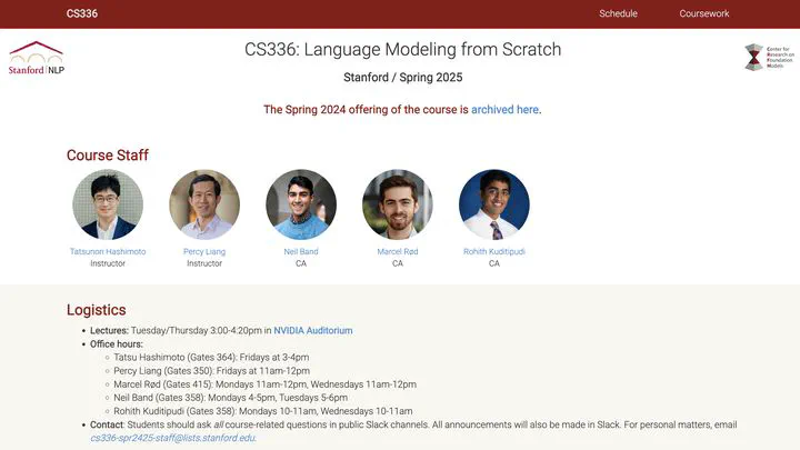 Image Credits: Screen capture of https://stanford-cs336.github.io/spring2025/ official website
“Language models serve as the cornerstone of modern natural language processing (NLP) applications and open up a new paradigm of having a single general purpose system address a range of downstream tasks. As the field of artificial intelligence (AI), machine learning (ML), and NLP continues to grow, possessing a deep understanding of language models becomes essential for scientists and engineers alike. This course is designed to provide students with a comprehensive understanding of language models by walking them through the entire process of developing their own. Drawing inspiration from operating systems courses that create an entire operating system from scratch, we will lead students through every aspect of language model creation, including data collection and cleaning for pre-training, transformer model construction, model training, and evaluation before deployment.” (Adapted from the official course website)
These are condensed notes from working through the course on my own: the points worth keeping from each lecture, with links to the original slides or lecture code and the Stanford recording. Lecture 01 is written up in more depth because it is where I started.
Lecture 01: Overview and Tokenization
Why this course?
- Modern researchers are disconnected from the tech stack (prompting > fine-tuning > training).
- Abstractions in LLMs are leaky and not well understood.
- The course teaches understanding through building: tokenizers, models, data pipelines, and training.
Scaling Laws:
- Goal: Predict optimal hyperparameters for large-scale models by experimenting at small scale.
- Given a FLOPs budget ($C$ ), find optimal model size ($N$ ) and data size ($D$ ).
- Rule of thumb: $D^* = 20N^*$ , from Kaplan et al., 2020 and Hoffmann et al., 2022.
- This is known as Chinchilla Optimality — doesn’t consider inference cost though!
Historical Context:
- Pre-2010s: Shannon’s entropy, n-gram models.
- 2010s: Neural LMs (Bengio, Attention, Transformer).
- 2018+: Pretrained models like BERT, GPT-2, T5.
- Modern: Scaling laws, alignment, mixture of experts, compute efficiency.
What we can learn:
- Mechanics: How transformers, parallelism, and tokenization work.
- Mindset: Think in terms of resources and efficiency.
- Intuition: Data/modeling decisions (some do not transfer across scale).
Tokenization
Goal: Convert raw text (Unicode strings) to sequences of integers (tokens) and back.
Why care?
- Poor tokenization increases sequence length (hurts compute).
- Good tokenization yields high compression, efficient training.
Tokenization Methods
Character-based:
- Each Unicode character becomes a token (e.g.,
🌍→ 127757). - Large vocab (~150k), poor compression.
- Each Unicode character becomes a token (e.g.,
Byte-based:
- Each byte (0–255) becomes a token via UTF-8.
- Fixed small vocab (256), but long sequences.
Word-based:
- Uses regex rules to segment strings into words.
- Vocabulary grows with corpus; OOV (out-of-vocab) issues.
Byte Pair Encoding (BPE):
- Merges frequent byte pairs iteratively.
- Trained on raw text; balances vocab size and sequence length.
- Used in GPT-2, GPT-3 tokenizers.
Observations
- GPT-2’s tokenizer merges frequently co-occurring byte pairs.
- Strings like
"hello world"get segmented into different tokens depending on context. - Special tokens (e.g.,
<|endoftext|>) must be preserved during encoding/decoding.
Key Takeaways
- BPE tokenization strikes a balance between efficiency and practicality.
- Tokenization deeply affects model size, training cost, and downstream performance.
- In this course, we’ll build a tokenizer from scratch and integrate it into our pipeline.
Additional Videos
Assignment 1 Solution
https://github.com/DhyeyMavani2003/stanford-cs336-assignment1-basics-solution/tree/main
Next up: PyTorch building blocks and efficient training routines.
Lecture 02: PyTorch and Resource Accounting
Two resources to track:
- Memory (GB) and compute (FLOPs); mechanics are just PyTorch, accounting is the habit.
- 70B params on 15T tokens is $6ND = 6.3 \times 10^{24}$ FLOPs: about 144 days on 1024 H100s at 50% MFU.
- Naive AdamW is 16 bytes/param (4 params + 4 grads + 4+4 optimizer state), so 8 H100s (640 GB) hold 40B, activations excluded. bf16 params/grads with an fp32 copy saves no memory, only time (Rajbhandari et al., 2019).
Float types:
- float32 is 4 bytes, so one GPT-3 feedforward matrix ($49152 \times 12288$ ) is 2.3 GB.
- float16 halves that but its low-end range is bad:
torch.tensor([1e-8], dtype=torch.float16)underflows to 0, where instability starts. - bfloat16 is 2 bytes with float32’s range, worse resolution; range matters more here. fp8 was standardized in 2022 (arXiv:2209.05433); H100 supports E4M3 and E5M2.
- Fix: mixed precision, bf16/fp8 for the forward pass and float32 for parameters and gradients (Micikevicius et al., 2017).
Tensors are pointers plus strides:
- Slicing,
view, andtransposereturn views on the same storage: free, but aliased, so mutating one mutates the other. - Non-contiguous views can’t be re-viewed;
.contiguous()copies, costing memory and compute. - Name dimensions instead of counting back from -1:
jaxtypingfor shapes,einsum/reduce/rearrangefor ops.
- Slicing,
FLOPs:
- A $(m \times n)(n \times p)$ matmul is $2mnp$ ; elementwise is $O(mn)$ , so for large matrices only matmuls count.
- Forward is $2 \cdot \text{tokens} \cdot \text{params}$ , backward $4$ (weight grad plus the grad passed down), total $6$ .
- A100: 312 teraFLOP/s bf16 vs 19.5 fp32. H100: 989.5 dense (1979 sparse) vs 67.5.
- MFU = actual over promised FLOP/s; $\geq 0.5$ is good. Measured bf16 MFU runs low; the promised number is optimistic.
- GPT-3 took 3.14e23 FLOPs; the revoked US executive order’s threshold was 1e26.
Initialization:
randnweights make each output element scale as $\sqrt{d_{\text{in}}}$ , which blows up gradients. Rescaling by $1/\sqrt{d_{\text{in}}}$ makes output scale invariant to fan-in: Xavier up to a constant (Glorot and Bengio, 2010), truncated to $[-3, 3]$ .
Training loop plumbing:
- Token ids are one flat array;
np.memmapit (LLaMA’s data is 2.8 TB), sampling random start offsets per batch. pin_memory()then.to(device, non_blocking=True)loads the next CPU batch while the GPU works.- Each optimizer adds one idea: momentum = SGD + exponential averaging of grad; AdaGrad = SGD + averaging by $g^2$ (Duchi et al., 2011); RMSProp = AdaGrad with exponential averaging; Adam = RMSProp + momentum.
- Per-step float32 memory is $4(\text{params} + \text{activations} + \text{gradients} + \text{optimizer states})$
. Seed torch, numpy, and
random; checkpoint model and optimizer state_dicts.
- Token ids are one flat array;
Lecture 03: Architectures, hyperparameters
Architecture
The framing:
- Low consensus except pre-norm, drifting toward LLaMA-like architectures. Over 19 new dense models last year, many only minor tweaks.
- What actually varies: position embeddings, activations, tokenization.
Pre-norm, universally:
- Set the norm off the main residual path. BERT was post-norm; OPT-350M is the odd modern exception.
- Originally sold as removing warmup; today the case is stability and larger LRs. Gradient attenuation Xiong et al., 2020, fewer gradient spikes (Salazar and Nguyen, 2019).
RMSNorm over LayerNorm:
- Drops mean subtraction and the bias term.
- The win is not FLOPs, since matmuls dominate those; it is data movement (Ivanov et al., 2023). FLOPs are not runtime. Bias terms go for the same reason.
Gated FFNs:
- Gating multiplies the first projection entrywise by an extra linear term $xV$ , so GLU variants scale $d_{ff}$ down by $2/3$ .
- Gains are consistent but small Shazeer, 2020, and GPT-3 did fine on plain GeLU.
RoPE:
- What you want: $\langle f(x,i), f(y,j)\rangle = g(x,y,i-j)$ . Sine embeddings leave cross terms; absolute ones obviously fail.
- Fix: pair up coordinates and rotate each 2D pair by position. Inner products are rotation invariant, so only $i-j$ survives Su et al., 2021, and it is reapplied at every attention op.
Hyperparameters
Shape defaults:
- $d_{ff} = 4 d_{model}$ , or $8/3$ with GLU; real GLU models run 2.5 to 4. T5 11B went to 64x before v1.1 walked it back to 2.5. Kaplan et al., 2020 finds a basin from 1 to 10.
- $n_{heads} \times d_{head} = d_{model}$ nearly everywhere. Papers argued against the 1-1 rule, but no low-rank bottleneck appears in practice.
- $d_{model}/n_{layers}$ anywhere in 100 to 200; systems concerns pick it, since deep models parallelize worse and add latency.
Regularization: dropout 0.1 in older models, weight decay near 0.1 alone in newer ones. The weight decay is not fighting overfitting, it interacts with the cosine LR schedule (Andriushchenko et al., 2023).
Stability and inference cost
- Softmaxes are where instability lives: z-loss on the output softmax (PaLM pioneered it), QK norm on queries and keys before the attention softmax, logit soft-capping via tanh.
- KV cache cost: training-time attention has high arithmetic intensity; incremental decoding does not, and the bad term scales like $n/d$ , hard to shrink. MQA keeps one key/value dimension, GQA interpolates: small perplexity hit for MQA Shazeer, 2019, little to none for GQA Ainslie et al., 2023.
- Restricting the pattern: sparse and sliding-window attention trade expressiveness for runtime Child et al., 2019, and depth extends the effective context (Mistral). Standard now interleaves: Command A makes every 4th layer full, long-range via NoPE, short-range via RoPE + SWA.
Lecture 04: Mixture of experts
- What a MoE is:
- Replace the big feedforward with many feedforwards plus a selector layer, so the expert count can grow without changing FLOPs per token.
- Upsides: same FLOPs with more parameters does better, MoEs are faster to train, and each expert FFN fits on one device, adding a parallelism axis (Fedus et al., 2022, OLMoE).
- Why they stayed niche: the infra is complex, the advantage shows up mainly multi-node, and the training objectives are heuristic and sometimes unstable.
Routing
- Top-k token choice:
- Almost every shipped MoE uses it.
- $k$ in practice: Switch Transformer 1, GShard / Grok / Mixtral 2, Qwen and DBRX 4, DeepSeek 7.
- Softmax placement differs: the DeepSeek V1-2 router (also Grok, Qwen) softmaxes before the top-k; Mixtral, DBRX and DeepSeek v3 after (Dai et al., 2024).
- Fine-grained plus shared experts:
- More and smaller routed experts, plus a few always-on shared ones. Used by DeepSeek and Qwen, originally from DeepSpeed-MoE.
- Routed / active / shared: DeepSeek v1 64/6/2 at fine-grained ratio 1/4, DeepSeek v3 256/8/1 at 1/14, OLMoE 64/8/0 at 1/8.
- DeepSeek’s ablations like both; OLMoE sees gains from fine-grained and none from shared.
Training
- The core problem:
- Sparsity buys training-time efficiency, but sparse gating decisions are not differentiable.
- Options: RL on the gating policy (REINFORCE, Clark et al., 2020, rare because of gradient variance), stochastic perturbation (Shazeer et al., 2017 adds Gaussian routing noise), heuristic balancing losses. Everyone uses the third.
- Load balancing:
- Efficiency needs experts used evenly. For the Switch aux loss, the derivative with respect to $p_i(x)$ scales with $\sum \mathbb{1}[\arg\max p(x) = i]$ , so more frequent use means stronger downweighting.
- DeepSeek v1-2 add per-device balancing on top of per-expert, v2 a communication balancing loss. DeepSeek v3 swaps those for per-expert biases updated online, called auxiliary-loss-free balancing, though a sequence-wise aux loss remains.
- Stability and fine-tuning:
- Run the expert router in float32, sometimes with a router z-loss (ST-MoE).
- Sparse MoEs overfit smaller fine-tuning sets. ST-MoE tunes only the non-MoE MLPs; DeepSeek throws data at it instead (1.4M SFT).
- Token dropping is batch-level:
- Another user’s query can drop your token. A proposed explanation for GPT-4’s nondeterminism.
- Upcycling:
- Init an MoE from a pre-trained dense checkpoint. Qwen MoE (from Qwen 1.8B, top-k 4, 60 experts, 4 shared) is one of the first confirmed successes.
- DeepSeek scale:
- v1 16B total / 2.8B active, v2 236B / 21B, v3 671B / 37B.
Lecture 05: GPUs
The machine
Execution model:
- CPUs optimize for a few fast threads, GPUs for many: tiny ALUs, little hardware for branching and control.
- Many SMs (streaming multiprocessors) independently execute blocks; each holds many SPs executing threads.
- A warp is 32 consecutively numbered threads executing together, same instruction on different inputs (SIMT). Conditionals are fine but carry real overhead.
- A thread sees its own registers and its block’s shared memory; crossing blocks means going through global memory.
Memory hierarchy:
- Closer to the SM is faster: L1 and shared memory inside it, L2 on die, global memory in the chips next to the GPU.
- SRAM is ~8x faster than DRAM and ~100x more expensive.
- Tensor cores (V and T series onward) are specialized matmul circuits: matmuls are >10x faster than other floating point ops.
Making ML workloads fast
Memory is the bottleneck:
- FLOPs scale faster than memory, so keeping the compute units fed is the hard part (Horace He).
Reduce memory accesses:
- Fusion: $\sin^2 x + \cos^2 x$
naively launches 5 CUDA kernels, shipping data back and forth. All 5 fuse into one, which
torch.compiledoes automatically. - Coalescing: DRAM is read in burst mode; accesses coalesce only when every thread in a warp falls in the same burst. For row-major matrices, threads moving along rows are not coalesced.
- Fusion: $\sin^2 x + \cos^2 x$
naively launches 5 CUDA kernels, shipping data back and forth. All 5 fuse into one, which
Move memory into shared memory:
- Tiling: non-tiled matmul reads each input $N$ times from global memory; tiling makes that $N/T$ from global plus $T$ within each tile, a factor of $T$ less global access.
- Wave quantization: with a $256 \times 128$ tile, 1792 wide is $7 \times 14 = 98$ tiles and 1793 is $8 \times 15 = 120$ ; an A100 has 108 SMs, so it cannot execute all 120 at once (thonking.ai).
Trade memory for compute:
- Low precision: fewer bits, fewer bytes to move. Elementwise ReLU is 1 read + 1 write, so intensity goes from 8 bytes/FLOP in fp32 to 4 in fp16.
- Recomputation: three stacked sigmoids cost 8 memory read/writes at very low arithmetic intensity; throwing the activations away and recomputing gets $5/8$ the memory accesses (min-cut recomputation).
Unpacking FlashAttention
Tiling the matmuls:
- Attention is 3 matmuls (K, Q, V) with a softmax in between. Figure 1 of Dao et al. is literally tiling for that matmul; the softmax is what resists.
Online softmax (Milakov and Gimelshein, 2018):
- Incrementally update the max and set up a telescoping sum, so the softmax comes out tile by tile.
- The forward pass is then tile-wise inner products, a fused exponential, and that softmax; the backward pass recomputes tile-by-tile.
Lecture 06: Kernels, Triton
A100 numbers worth remembering:
- 108 SMs. DRAM 80GB (big, slow), L2 cache 40MB, L1 192KB per SM (small, fast). A block shares 164KB as fast as L1; threads synchronize only within a block.
- Thread blocks hit SMs in waves; the last wave is partly filled, so SMs idle. Rule of thumb: number of thread blocks $\geq 4\times$ the number of SMs.
- Arithmetic intensity = FLOPs / bytes: high is compute-bound (good), low is memory-bound (bad). Matmul is compute-bound, everything else memory-bound.
Benchmark and profile:
- Warm up first (the first call pays compilation and cold caches),
torch.cuda.synchronize()before stopping the clock, several trials for variance. - Benchmarking gives end-to-end time: compare implementations, watch scaling. Profiling tells you what is actually being called, down to names like
cutlass_80_simt_sgemm_256x128_8x4_nn_align1(CUTLASS, 256x128 tile).
- Warm up first (the first call pays compilation and cold caches),
Kernel fusion:
- From Horace He: warehouse is DRAM, factory is SRAM, so unfused ops each make the round trip; fused ones read and write once. Manual GeLU profiles as a stack of elementwise kernels,
F.geluas one. - Five ways to write a function: manual, PyTorch,
torch.compile, CUDA, Triton. For GeLU, hand-written CUDA beat manual but not PyTorch; Triton landed near PyTorch, behind the naive CUDA kernel.
- From Horace He: warehouse is DRAM, factory is SRAM, so unfused ops each make the round trip; fused ones read and write once. Manual GeLU profiles as a stack of elementwise kernels,
CUDA vs Triton:
- CUDA: write
f(i)for one thread, indexed byblockIdx/blockDim/threadIdx. Fine for elementwise; anything reading multiple values (matmul, softmax, RMSNorm) means hand-managing shared memory. - Triton (OpenAI, 2021) automates coalescing, shared memory, and scheduling within an SM; across SMs stays manual. Thinking in blocks, not threads, is what lets the compiler add thread coarsening: in the generated GeLU PTX one thread handles 8 elements.
- CUDA: write
Minimize reads and writes:
- Naive row-wise softmax (max, subtract, exp, sum, divide) costs $5MN + M$
reads and $3MN + 2M$
writes against a floor of $MN$
each, a 4x speedup left on the table. The Triton version: one block per row,
BLOCK_SIZE = next_power_of_2(N), write back once. - Naive matmul: $MKN$ reads, versus $MK + KN$ with A and B in shared memory (~10x faster, ~100KB), so big matrices get tiled block by block, writing partial sums. Block order matters for L2: the same 9 elements cost 90 loads one way, 54 the other.
- Write your own matmul for fusion with what comes next, e.g.
gelu(A @ B). The gap between the programming model (PyTorch, Triton, PTX) and the hardware is where performance mysteries live.
- Naive row-wise softmax (max, subtract, exp, sum, divide) costs $5MN + M$
reads and $3MN + 2M$
writes against a floor of $MN$
each, a 4x speedup left on the table. The Triton version: one block per row,
Lecture 07: Parallelism
Why parallelism:
- A single GPU cannot fit most large models. What we want from many is linear scaling in max params and model FLOPs.
- An all-reduce is a reduce-scatter plus an all-gather, and in the bandwidth-limited regime that is optimal. Every ZeRO stage exploits it.
Data parallel and ZeRO:
- Naive DP splits the batch: compute scales, communication is $2\times\#\text{params}$ per batch, memory does not scale, and machine count must stay below batch size.
- Mixed-precision Adam needs 16 bytes/param: 2 (BF16 params) + 2 (BF16 grads) + 4 (FP32 master weights) + 4 + 4 (Adam moments).
- ZeRO 1 shards optimizer state, 2 also gradients, 3 (FSDP) parameters too, requesting and freeing them as it steps through the graph.
- Stages 1 and 2 cost $2\times\#\text{params}$ , same as DDP, so they are effectively free. Stage 3 costs $3\times\#\text{params}$ , its extra all-gathers overlap with forward compute (FSDP paper, PyTorch tutorial).
- Pure BF16 with Kahan summation is 12 bytes/param. On 8x A100 80G: 6.66B params baseline, 16B at stage 1, 53.33B at stage 3.
Model parallel:
- Splits params like ZeRO 3 but communicates activations, and unlike ZeRO 3 it cuts activation memory too.
- Naive layer-wise splitting leaves each GPU active $1/n$ of the time. Micro-batched pipelining fixes that, bubble ratio $(n_{\text{stages}}-1)/n_{\text{micro}}$ , so pipelines need big batches.
- Tensor parallel cuts along width: each GPU gets columns of $A$ and rows of $B$ , with an all-reduce to recombine. No bubble, no batch-size dependence.
- The tradeoff is bandwidth: TP all-reduces $8bsh(n-1)/n$ per layer, a pipeline sends $bsh$ point-to-point per micro-batch. So TP intra-node (up to 8 GPUs), pipeline across nodes.
Activation memory and sequence parallel:
- After TP, $10sbh$ per layer remains (Korthikanti et al., 2022): LayerNorm $4sbh$ , dropout $2sbh$ , attention and MLP inputs $4sbh$ . The quadratic $5as/h$ term recomputes away, as in flash attention.
- Those are all pointwise over the sequence, so shard LayerNorm and dropout along the sequence axis. That is what finally makes memory linear.
3D parallelism:
- TP up to GPUs per machine, pipeline across machines (or ZeRO 3, depending on bandwidth), then data parallel with the rest. Gradient accumulate if the batch is small.
- Narayanan 2021: TP caps out at 8, PP grows to make the model fit, DP shrinks with scale (32 down to 6 at the largest). Across 64 machines, 8x8 is best.
- Real runs: Dolma 7B is FSDP alone; DeepSeek V3 is ZeRO 1 + PP=16 + 64-way expert parallel; Gemma 2 is ZeRO 3 + MP + DP.
Lecture 08: Parallelism
Setting:
- Last lecture: inside one GPU. This one: across GPUs and nodes. Same theme, since compute sits far from its data: inside a GPU you cut memory accesses with fusion and tiling, across GPUs you cut communication with replication and sharding.
- Hierarchy, small/fast to big/slow: L1 and shared memory, HBM, NVLink (intra-node), NVSwitch (inter-node).
Collective operations:
- Primitives from the 1980s parallel-programming literature: declare a pattern over all ranks instead of managing point-to-point sends. World size is the device count, rank is one device.
- $\text{all-reduce} = \text{reduce-scatter} + \text{all-gather}$ , shown by running the two in sequence over 4 ranks.
Hardware numbers:
- At home, GPUs on a node share a PCIe bus (v7.0, 16 lanes, 242 GB/s) and nodes talk over Ethernet at roughly 200 MB/s. In the data center, NVLink bypasses the CPU within a node and NVSwitch bypasses Ethernet across nodes.
- An H100 has 18 NVLink 4.0 links, 900 GB/s total; HBM on the same chip is 3.9 TB/s, so even the good interconnect is over 4x slower than local memory.
- NCCL detects the topology, optimizes the GPU-to-GPU path, and launches the kernels that move bytes.
ncclfor GPU,gloofor CPU.
Benchmarking collectives:
- Warmup call first, then
torch.cuda.synchronize()anddist.barrier()around the timed region; without both you time kernel launches. - All-reduce sends $2(W-1)$ times the tensor size (input out, output back), reduce-scatter only $(W-1)$ times its input. Effective bandwidth is those bytes over $W \times \text{duration}$ (nccl-tests).
- Warmup call first, then
Data parallelism (batch):
- Every rank holds all parameters and its own optimizer state. The only delta from single-GPU training is one
all_reducewithReduceOp.AVGover eachparam.gradafter backward. - Losses differ per rank (local data); gradients come out identical, so parameters stay in sync.
- Every rank holds all parameters and its own optimizer state. The only delta from single-GPU training is one
Tensor parallelism (width):
- Each rank gets $d/W$ columns of every layer, computes its slice of the activations, then all-gathers and concatenates on the feature dim before the next layer. Communication on every layer; all activations move.
Pipeline parallelism (depth):
- Each rank owns $L/W$
consecutive layers and uses
send/recvto its neighbor. Micro-batches shrink the bubble, but the bare version does not overlap communication with compute, so it stays.
- Each rank owns $L/W$
consecutive layers and uses
Loose ends:
- Skipped: attention, and real communication/compute overlap. Sequence (length) and expert (width) are the other axes.
- Jax/TPU alternative: define the model and the sharding strategy, let the compiler do the rest (Levanter).
- The three choices are always: re-compute it, store it in memory, or store it in another GPU’s memory and communicate.
Lecture 09: Scaling laws
- The setup:
- Ten thousand H100s for a month, one good open-source LM to build. Infra is A2, data A4; the open question is which model do you run.
- Old and unpleasant: tune hyperparameters on the big model. New (over?)optimism: tune on small models and extrapolate.
Data scaling
The empirical fact:
- Loss vs dataset size is linear on a log-log plot: a power law, “scale-free” (Kaplan et al., 2020). Same shape in machine translation, speech, and LM (Hestness et al., 2017).
Why a power law:
- Estimation error decays polynomially. Mean estimation gives $E[(\hat\mu - \mu)^2] = \sigma^2/n$ , i.e. $\log(\text{Error}) = -\log n + 2\log\sigma$ , and any rate $1/n^\alpha$ is a scaling law.
- Classical models mostly scale as $1/n$ , predicting slope $-1$ . Measured neural exponents look nothing like that.
- Flexible nonparametric learning has dimension-dependent exponents ($n^{-1/d}$ in $d$ dimensions); Bahri et al., 2021 tie $\alpha$ to the data’s intrinsic dimension, though those estimators are sketchy.
Composition and repetition:
- Data composition (train $\neq$ test) moves the offset, not the slope: hence diverse data.
- Repeated tokens are worth less than unique ones, so data selection should be scale-adaptive.
Model scaling
- The procedure:
- Fit a law per design choice from a few small models: optimizer (Adam vs SGD), architecture (transformer vs LSTM), depth. Beats spending tens of millions on an LSTM GPT-3.
- What the laws say:
- 1 vs 2 layers is a huge difference; more layers diminish below $10^7$ params; embedding parameters behave differently.
- Critical batch = min examples for a target loss / min steps for it; smaller target, bigger batch.
- Optimal LR moves with scale, so initialization and LR must be scale-aware ($\mu$ P, Yang et al., 2022).
- Upstream loss scales predictably; downstream performance often does not (Tay et al.).
Joint laws and Chinchilla
- Joint data-model fits:
- Rosenfeld et al., 2020 fit $\text{Error} = n^{-\alpha} + m^{-\beta} + C$ from small models and small data; you then optimize it against your costs.
- Hoffmann et al., 2022 argue those fits are off, mainly for ignoring LR schedules. Their three fits: min over the union of all training curves; IsoFLOPs (fix FLOPs, sweep params, minima form a power law); joint least-squares over a size-data grid.
- The first two mostly agree; the third was likely flawed, and Besiroglu et al., 2024 refit the recovered data to match them.
- Train-optimal is not deployment-optimal:
- Chinchilla optimizes fixed training compute, but most deployment compute is inference, so overtrain. Tokens per param: GPT-3 2, Chinchilla 20, LLaMA 65B 22, Llama 2 70B 29, Mistral 7B 110, Llama 3 70B 215.
Lecture 10: Inference
- Inference vs training:
- Training is a one-time cost; inference repeats on every request, plus evaluation, test-time compute, and RL sample generation.
- Training parallelizes over the sequence; generation is sequential, so compute goes underused.
Arithmetic intensity
- The 295 number:
- H100: $989 \times 10^{12}$ FLOP/s over $3.35 \times 10^{12}$ bytes/s, so accelerator intensity is 295.
- For $X (B \times D)$ times $W (D \times F)$ with $B \ll D, F$ , intensity collapses to $B$ : compute-limited iff $B > 295$ .
- Naive generation costs $O(T^3)$ FLOPs; the KV cache trades that for $S \cdot KH \cdot L \cdot 2 \cdot 2$ bytes per sequence (key + value, bf16).
- Prefill vs generation:
- MLP intensity is $BT$ : prefill ($T = S$ ) is easy to make compute-limited, generation ($T = 1$ ) rests on $B$ alone (concurrent requests).
- Attention intensity is $ST/(S+T)$ : $S/2$ at prefill, below 1 at generation, with no $B$ in it, so batching does not help. MLP weights are shared across the batch; KV caches are not.
- Llama 2 13B on an H100 at $S = 1024$ : 26 GB of weights, 0.84 GB of KV cache per sequence. $B = 1$ is ~8 ms/token, $B = 64$ ~24 ms/token, $B = 256$ needs 241 GB, will not fit. Small batches for TTFT, large for throughput.
Lossy shortcuts
- Shrink the KV cache:
- GQA: $N$ query heads, $K$ KV heads, cache shrinks by $N/K$ . Llama 2 13B at $K = 8$ instead of 40 gives 0.17 GB per sequence, buying back batch size.
- MLA: project K and V down to $C$ dims. DeepSeek v2 takes $NH = 16384$ to 512, plus 64 RoPE dims (MLA is not RoPE-compatible).
- CLA shares KV across layers; local attention makes the cache length-independent, interleaved with global layers (character.ai: 1 global in 6).
- Spend fewer bits:
- LLM.int8() pulls outlier dimensions into fp16, 15-23% slower; AWQ keeps 0.1-1% of weights high-precision by activation: int3, 4x less memory, 3.2x speedup.
- Prune then distill: score layers, heads, and dims on 1024 calibration samples, cut, distill back.
Lossless and dynamic
- Speculative sampling:
- Checking is faster than generating: draft model $p$ guesses ~4 tokens, target $q$ scores them in parallel (speculative decoding). Modified rejection sampling on residual $\max(q-p, 0)$ , always emitting one token, keeps the output an exact sample from $q$ .
- Pairings: 70B target with 8B draft, 8B with 1B. Medusa and EAGLE improve the draft side.
- Serving ragged traffic:
- Orca: iteration-level scheduling admits requests mid-decode; selective batching runs attention per sequence, concatenating the rest.
- PagedAttention: non-contiguous KV cache blocks, killing fragmentation and sharing prefixes copy-on-write.
- SSMs replace the $O(T)$ KV cache with $O(1)$ state (Mamba, Jamba), weak at associative recall, so strong models keep some full attention.
Lecture 11: Scaling laws
Scaling recipes in the wild
The question:
- Does Chinchilla’s recipe work in practice, can fitting it be made cheaper, and do some parametrizations scale better?
- Only Cerebras-GPT, MiniCPM, and DeepSeek publish detailed recipes; LLaMA 3, Hunyuan-1, MiniMax-01 are newer but thinner.
Cerebras-GPT:
- 0.1B to 13B models, Chinchilla formula applied directly. Core finding: muP scales more predictably.
- Stable constants:
scale_emb = 10,lr = 6e-3,init_base = 0.08.
MiniCPM:
- 1 to 2.5B models that beat most 2Bs and match many 7Bs. Constants:
scale_emb = 12,scale_depth = 1.4,init_std = 0.1,lr = 0.01. - muP for initialization, fix the aspect ratio, scale the size. Batch, LR, and token-to-size ratio are each fitted by scaling analysis.
- Batch sweeps at 9M, 30M, 170M: the minimum-loss point per data size is the optimal batch, and plotted against final loss as in Kaplan et al., 2020 it grows polynomially as loss falls.
- Their largest scaling run is only ~5x smaller than the model they shipped.
- 1 to 2.5B models that beat most 2Bs and match many 7Bs. Constants:
Making the Chinchilla sweep affordable:
- Chinchilla needs each point trained from scratch, not early-stopped, taking a fit from $n$ to $n^2$ .
- WSD (warmup, stable, decay) lets you restart at the end of the stable phase; decay is ~10% of the run, where loss drops fast. DeepSeek uses two 10% decay steps and matches cosine.
Ratios keep climbing:
- MiniCPM’s joint fit (method 3) gives 192 tokens per parameter, far past $D^* = 20N^*$ . LLaMA 3 reports 39-to-1 from isoflops, Hunyuan-1 96-to-1 against active params for an MoE.
- DeepSeek skips muP: assume most hypers are scale-invariant, pick batch and LR from small runs within 0.25% of min loss, then isoflops for sizing.
muP, derived and stress-tested
Two conditions:
- A1: activations at initialization stay $\Theta(1)$ , so the hidden norm is $\Theta(\sqrt{n_l})$ . A2: after one gradient step the change in activation is also $\Theta(1)$ .
- For a deep linear net these pin initialization to $\Theta\left(\frac{1}{\sqrt{n_{l-1}}}\min\left(1, \sqrt{n_l/n_{l-1}}\right)\right)$ and SGD LR to $\Theta(\sqrt{n_l/n_{l-1}})$ ; under Adam, $\Theta(1/n_{l-1})$ .
- Against standard parametrization ($1/\sqrt{n_{l-1}}$ init, $\Theta(1)$ LR) the real differences are the Adam LR and the init when fanout is below fanin.
- Width only; depth is not handled.
What it survives:
- SwiGLU and squared ReLU, same optimal LR. Large and small batch, never addressed in the derivation. SP vs muP unembedding, zero-query init.
What breaks it:
- Learnable RMSNorm gains, which can be removed with little loss of performance. Sign-based optimizers like Lion. Strong (0.1) weight decay, maybe the only significant failure.
- Still worth using, mainly because standard parametrization is quite a bit more unstable.
Lecture 12: Evaluation
What evaluation is for:
- Given a fixed model, how good is it? There is no one true evaluation; it depends on the question: a purchase decision, raw capability, benefits and harms for business and policy, or developer feedback.
- Framework: what are the inputs, how do you call the model, how do you score the outputs, how do you interpret the number.
- With chain-of-thought, tools and RAG in play you are evaluating an agentic system, not a model. Model developers want the former, users want the latter.
Perplexity:
- $(1/p(D))^{1/|D|}$ measures whether $p$ puts high probability on a dataset $D$ .
- Old papers trained and tested on splits of one corpus (Penn Treebank, WikiText-103, One Billion Word). GPT-2 scored them zero-shot, out-of-distribution; transfer helped on the small sets, not on 1BW.
- Still worth tracking: smoother than downstream accuracy (good for fitting scaling laws) and universal.
- Maximalist view: the floor is $H(t)$ , hit only at $p = t$ , and with $t$ you solve every task.
Benchmarks worth knowing:
- MMLU: 57 subjects, multiple choice. A knowledge test, not language understanding. MMLU-Pro strips noisy and trivial items and goes 4 to 10 choices; scores drop 16-33%.
- GPQA: written by 61 PhD contractors. PhD experts 65%, non-experts 34% with Google and 30 minutes, GPT-4 39%.
- AlpacaEval: 805 instructions, win rate against GPT-4 preview as judged by GPT-4 preview (bias baked in). WildBench: 1024 prompts from 1M real conversations, 0.95 correlation with Chatbot Arena.
- Agent = model + scaffolding. SWE-Bench: 2294 tasks over 12 Python repos, graded by unit tests. CyBench: 40 CTFs, difficulty from first-solve time.
- HarmBench: 510 harmful behaviors. AIR-Bench: 314 risk categories, 5694 prompts from regulation and company policy. GCG optimizes prompts that bypass safety and transfer from open weights (Llama) to GPT-4.
What bites:
- Safety splits into capability and propensity: propensity matters for API models, capability for open weights where fine-tuning strips refusals. CyBench is run as a safety eval but is arguably a capability eval.
- Quizzing prompts (user knows the answer) fill benchmarks; asking prompts are the realistic ones, where user value is.
- Train-test overlap is the validity problem now that training data is undisclosed; labels are noisy too, hence SWE-Bench Verified and Platinum benchmarks.
- Old work evaluated methods on fixed splits; we now evaluate models/systems. The nanogpt speedrun (fixed data, time to a target validation loss) and DataComp-LM (fixed training pipeline, optimize the data) are the exceptions.
Lecture 13: Data
Data is the part nobody publishes:
- Llama 3 documents architecture and training procedure in full and says nothing about data. Two reasons: competitive dynamics and copyright liability.
- Data does not fall from the sky: a long-tail problem that scales with human effort, unlike architecture or systems.
- Pre-training on raw web text, mid-training on high-quality data for capabilities, post-training on instruction data or RL: lots of low-quality data to a little high-quality data. Base model = through mid-training, instruct/chat = after post-training.
Common Crawl plumbing:
- ~100 crawls since 2008. WARC is the raw HTTP response, WET is pre-converted text and that conversion is lossy.
- DCLM shows the HTML-to-text conversion moves downstream accuracy, so start from WARC and run trafilatura or resiliparse yourself.
The filtering lineage:
- C4 is hand rules only: keep lines ending in punctuation with $\geq 5$
words, drop pages under 3 sentences or containing
{or bad words. One April 2019 snapshot of 1.4T tokens became 156B. - Gopher’s MassiveWeb added rules like “80% of words contain at least one alphabetic character”. 10.5 TB collected, trained on 300B of it, about 12%.
- RefinedWeb avoided ML-based filtering on purpose, to dodge classifier bias; FineWeb extended that line to 15T tokens.
- DCLM-baseline went the other way: a fastText classifier trained on 200K positives (OpenHermes-2.5, ELI5) against 200K negatives (RefinedWeb), run over the 240T-token pool, yielding 3.8T that beat the other filtering methods.
- Nemotron-CC argues DCLM and FineWeb-Edu filter too hard, removing 90% of the data. It ensembles classifiers and rephrases weak documents with an LM instead of discarding them: 6.3T tokens, 1.1T high-quality. Llama 3 trained on 15T, Qwen3 on 36T.
- C4 is hand rules only: keep lines ending in punctuation with $\geq 5$
words, drop pages under 3 sentences or containing
Copyright:
- The threshold is extremely low, so most of the internet is copyrighted, and it covers expression rather than ideas.
- Copying the data is a violation before you train on anything, so you either license it or appeal to fair use. Training is plausibly transformative, but the exposure is factor four, effect on the market. Terms of service bind on top.
Mid- and post-training:
- Attention is quadratic, so extend context later rather than pre-train long. LongLoRA takes Llama 2 7B from 4K to 100K with shifted sparse attention and positional interpolation, trained on PG-19 and Proof-Pile.
- Llama 2 chat used 27,540 vendor-annotated examples and reported that beat the millions of examples in open datasets.
Lecture 14: Data
Filtering algorithms
The problem:
- Given target data T and lots of raw data R, find the subset of R similar to T. Must generalize past T and be fast enough to run over all of R.
One framework, three scores:
- Generative model of T: $p_T(x)$ , keep above a threshold. KenLM n-grams with Kneser-Ney smoothing, so just count and normalize. Fast but crude.
- Discriminative classifier: $p(T \mid x)$ . fastText averages word embeddings before the head, so $H(V+K)$ parameters instead of $VK$ ; bigrams go through the hashing trick, 10M bins. For good versus bad, $H = K = 2$ and it is just a linear classifier.
- Importance resampling: $p_T(x)/p_R(x)$ , resample proportional to score. DSIR fits hashed n-gram models on both sides, since T is too small for anything richer. Slightly better than fastText on GLUE.
- Items are paragraphs, sorted by increasing KenLM perplexity, keep the top 1/3. Used in LLaMA.
Applications
Language ID:
- fastText
lid.176off the shelf, 176 languages. Dolma keeps pages with $p(\text{English}) \geq 0.5$ . - Weak on short sequences, low-resource and similar languages (Malay/Indonesian), and code-switching. Can quietly drop dialects of English.
- fastText
Quality:
- C4, Gopher, RefinedWeb, FineWeb and Dolma use no model-based filtering; GPT-3, LLaMA and DCLM do.
- GPT-3 scored CommonCrawl against positives from Wikipedia, WebText2 and Books, then kept documents stochastically with a Pareto draw rather than a hard cut. LLaMA/RedPajama used pages referenced by Wikipedia as positives.
- phi-1: GPT-4 labels a 100K subset of The Stack’s Python for educational value, a random forest over codegen embeddings extrapolates. A 1.3B model hits 17.68% on HumanEval after 36K filtered steps, versus 12.19% after 96K unfiltered.
Toxicity:
- Dolma trains two fastText classifiers on the Jigsaw toxic comments data: hate and NSFW.
Deduplication
Why:
- Fewer tokens, and less memorization, which mitigates copyright and privacy. One product description appears 61,036 times in C4.
Design space:
- What counts as an item, how to match, what to drop. C4 exact-matches 3-sentence spans; cutting one from the middle can leave the document incoherent.
Bloom filter:
- $k$ hashes into $m$ bins gives $f = (1 - (1 - 1/m)^{kn})^k$ . More bins alone only buys $O(1/m)$ ; optimal $k = \ln 2 \cdot m/n$ gives $f = 0.5^k$ , exponential in compute. Dolma targets $10^{-15}$ over paragraphs.
MinHash and LSH:
- Min hash over a set’s elements, so $\Pr[h(A) = h(B)] = \text{Jaccard}(A,B)$ .
- Split $n = br$ minhashes into $b$ bands of $r$ , collide if all of some band matches: $1 - (1 - s^r)^b$ . The and-or structure sharpens that into a near-threshold at $(1/b)^{1/r}$ . Deduplicating training data uses n = 9000, b = 20, r = 450.
Lecture 15: Alignment - SFT/RLHF
- The framing:
- Pretraining gets you GPT-3, not InstructGPT; deployment needs tighter output control. Recipe: SFT then RLHF, from Ouyang et al., 2022.
- SFT fits $\hat{p}(y \mid x) \approx p^*(y \mid x)$ , needing samples from the reference policy. RLHF finds $\hat{p}$ maximizing $E_p[R(y,x)]$ : the LM becomes a policy, not a model of a distribution.
SFT
What is in the data:
- FLAN (academic NLP tasks reformatted), Alpaca (short, simple instructions), OpenAssistant (long human answers with references). They vary in length, style, references, scale, and safety.
- Preference evaluation has strong length effects, human and GPT judges alike (Dubois et al., 2023), though style barely moves benchmarks.
Knowledge:
- Folklore: fine-tuning on facts the model does not know makes it hallucinate (Schulman, 2023; Gekhman, 2023); maybe skip tail knowledge.
- SFT works best extracting pretraining behaviors, not adding new ones; even factually correct data can hurt.
Safety:
- ~500 Alpaca-style examples moves a safety profile; the hard part is over-refusals.
Midtraining:
- Pretrain on web data, mix instruction data in, then a short SFT round: scale instruction tuning without catastrophic forgetting. Undocumented but common; publicized in miniCPM, jetMoE.
RLHF
Why optimize:
- 7B model: ~$25k annotation for demonstrations vs ~$4k for pairwise feedback, against ~$300k of base-model compute.
- People do not always write what they prefer in LM outputs (Zhang et al., 2023).
Data:
- InstructGPT: 40 crowdworkers via Scale and Upwork. Annotator distribution shifts behavior (Santurkar et al., 2023) and style (Hosking, Blunsom, Bartolo, 2024).
- GPT-4 is a good pairwise judge: near-perfect system-level rank correlation, agreement near human inter-annotator levels, hence cheap AI feedback (UltraFeedback, Zephyr 7B, Tulu 3).
PPO in three steps:
- $\nabla_\theta E_{p_\theta}[R(z)] = E_{p_\theta}[R(z)\nabla_\theta \log p_\theta(z)]$ , variance too high; TRPO linearizes around the current policy; PPO clips the ratios at some $\epsilon$ . Finicky in practice.
DPO:
- Drop the reward model and on-policy machinery: assume $\pi$ is all policies (links policy and reward in closed form), parametrize the reward via the policy, optimize with the Stiennon et al., 2020 pairwise objective.
- Reduces to a positive gradient on chosen, negative on rejected, scaled by the implied reward’s prediction error.
- Matched the lecture’s own PPO in simulation with none of the pain, though PPO sometimes wins. Variants (Tulu 3): SimPO (no reference model), length-normalized DPO.
Failure modes:
- Overoptimization: past some point, optimizing reward overfits it, for human and noisy LM preferences but not noiseless ones.
- Mode collapse: an RLHF’d model is no longer probabilistic, so no calibration. Length inflation is the other big outcome (Chen et al., 2024; Singhal et al., 2024).
Lecture 16: Alignment - RL
DPO, finishing last lecture:
- No reward model, no rollouts: step up on good completions, down on bad, weighted by the implied reward model’s prediction error.
- Assuming $\pi$ ranges over all policies gives the implied reward in closed form, and the Stiennon pairwise objective fits it. Same simulated performance as AlpacaFarm’s PPO, none of the pain.
Why leave RLHF:
- Overoptimization: past a point, optimizing the reward overfits it. True for human and noisy LM preference, not noiseless.
- Mode collapse: RLHF’d models are no longer probabilistic models, so no calibration.
- Hence verifiable rewards: optimize exactly what you want, in narrow domains.
PPO:
- Policy gradient variance is too high; TRPO linearizes around the current policy; PPO clips the ratio (cliprange 0.2).
- Per-token KL penalty, full reward on the last token, KL clipped where new logp falls below the reference. GAE with $\gamma = \lambda = 1$ works because this is a bandit problem.
- The value model is why people move on: memory hungry, extra tuning.
GRPO:
- PPO minus the value function; advantage is a z-score inside the rollout group. Online it is just policy gradient with group-normalized rewards, hence the tiny implementations.
- Dividing by that std is not a valid baseline: only state-dependent terms keep the gradient unbiased (Sutton and Barto). It upweights too-easy and too-hard questions, and the length normalizer adds length bias; Dr. GRPO (Liu et al., 2025) fixes both.
Case studies
R1:
- R1-zero is pure GRPO on DeepSeek-V3 with accuracy and format (thinking tag) rewards. CoTs lengthen and the “aha moment” shows up, but Dr. GRPO credits the length to the biased objective, and the base model already does “aha”.
- R1 adds SFT init, a language-consistency reward, non-verifiable rewards, then 2 epochs of SFT (600k V3-judged non-verifiable samples, 200k non-reasoning) and GRPO again for RLHF. 800k traces distilled into Qwen 2.5. PRMs and MCTS are in the unsuccessful-attempts section.
Kimi K1.5:
- Reference-based reward model and a DPO-style derivation with a squared-loss surrogate, so no GRPO length bias.
- Keep only problems failed at best-of-8, drop multiple choice, sample proportional to (1 - success rate). Length reward with $\lambda \in [-0.5, 0.5]$ , enabled late: correct answers pushed short, wrong ones below the middle of the rollouts.
Qwen 3:
- Same playbook, then GRPO on 3995 examples after dropping anything solvable without CoT.
- General RLHF after reasoning RL costs some math/STEM.
RL infra:
- Rollouts mean slow inference, train and rollout stacks differ, long CoTs make batches uneven.
Lecture 17: Alignment - RL
RL setup for a language model:
- State $s$ is the prompt plus response so far, action $a$ the next token, policy $\pi(a \mid s)$ just a fine-tuned LM.
- Transitions are deterministic ($s' = s + a$ ), so unlike robotics you can plan and spend test-time compute.
- Rewards here are outcome (depend on the whole response) and verifiable (deterministic), so discounting and bootstrapping matter much less.
Policy gradient:
- Writing $a$ for the entire response, $\nabla E[R] = E[\nabla \log \pi(a \mid s) R(s, a)]$ , so the naive update is SFT weighted by reward.
- With $R \in \{0, 1\}$ it only updates on correct responses: SFT on a dataset that shifts as the policy shifts.
- Variance is the problem: verifiable rewards are sparse, where RLHF preference-trained reward models are more continuous.
Baselines:
- Maximizing $E[R - b(s)]$ shifts the objective by a constant independent of $\pi$ , so the estimate stays unbiased.
- Two states: $s_1$ pays 11 and 9, $s_2$ pays 0 and 2. Raw rewards rank the 9 above the 2, even though the 2 is the better action at its own state. Baselines $b(s_1) = 10, b(s_2) = 1$ drop the update signal’s std from 5.323 to 1.155.
- The optimal $b^*(s)$ is hard to compute, so the heuristic is the mean reward $b(s) = E[R \mid s]$ , which makes the baselined reward the advantage $A(s,a) = Q(s,a) - V(s)$ , with $Q = R$ here because $a$ is the whole response.
GRPO mechanics:
- DeepSeekMath, 2024 drops the critic from PPO, 2017 and uses the group of responses sampled per prompt as the baseline.
- Choices of $\delta$ to update on: raw rewards, centered (minus group mean), normalized (divided by group std), max-only (zero all but the best).
- Loss variants: naive log-prob weighting, the importance ratio $\pi / \pi_{old}$ , the clipped ratio (lecture code uses $\epsilon = 0.01$ ).
- Gotcha: compute $\pi_{old}$
under
torch.no_grad(), or the ratio differentiates through both halves and the gradient is exactly 0. - Optional KL penalty against a frozen reference model, estimated as $E_p[q/p - \log(q/p) - 1]$ , for adding a capability without losing old ones.
What the sorting demo shows:
- Task: sorting 3 numbers, one point per prompt token present in the response plus one per adjacent sorted pair: more partial credit than counting matched positions.
- Raw rewards, 100 epochs of 10 steps with 10 responses per prompt: still has not learned to sort, on the training prompts.
- Centering helps: suboptimal responses get a negative update, and a prompt whose responses all tie produces none. Still lands in local optima.
- Dividing by the group std changes little; Dr. GRPO, 2025 drops it to avoid length bias, moot when all responses are one length.
Lectures 18 and 19: guest lectures
No public materials.
Lecture 18 (Junyang Lin) and Lecture 19 (Mike Lewis) were guest talks. The course schedule lists no slides or code for either, and Stanford Online’s Spring 2025 playlist stops at Lecture 17, so there is nothing public to take notes from. Leaving these blank rather than reconstructing them from memory.
Assignments
Five assignments, each building on the last. Handouts and starter code are public.
- A1 - Basics: implement the tokenizer, model architecture and optimizer, then train a small Transformer LM. My solution.
- A2 - Systems: profile and benchmark A1’s model, write your own Triton FlashAttention-2, and build a memory-efficient distributed version of the training code.
- A3 - Scaling: query a training API and fit a scaling law to project model scaling.
- A4 - Data: turn raw Common Crawl dumps into usable pretraining data through filtering and deduplication.
- A5 - Alignment and reasoning RL: supervised finetuning plus RL to get an LM to reason through math problems. Optional second part implements DPO.
If you are following along outside Stanford, the course notes that a single H100 runs roughly $2-3/hour on RunPod, Lambda, or Paperspace, and recommends debugging on CPU first.